Stability of the excavation base in relation to solid pipping erosion
The excavation bottom tool allows for the determination of the safety factor concerning the stability of the excavation bottom (solid pipping erosion).
General presentation
Principle
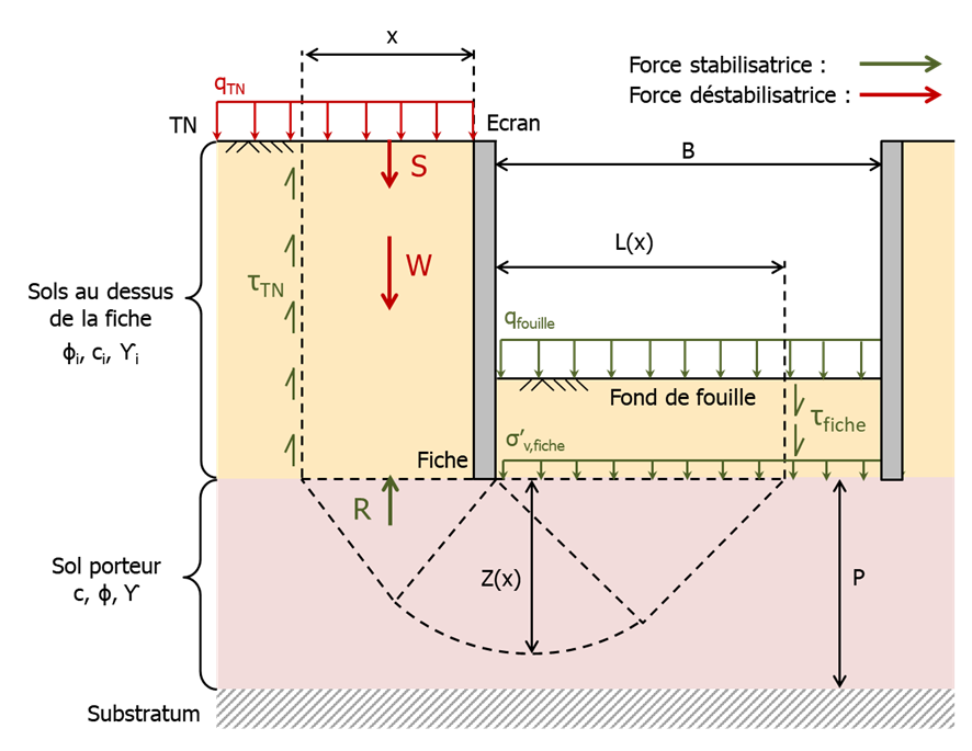
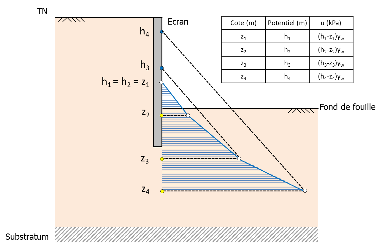
The verification is summarized according to the mechanism represented in the following figure, defining stabilizing and destabilizing forces.
The tool seeks the value of \(x\) such that the safety factor \(F(x)\) is minimized, where \(F(x)\) is given by:
where :
- \(S(x)\) : Destabilizing force linked to the overload on the GL side (\(kN/ml\)) :
- \(W(x)\) : Destabilizing force related to the weight of the GL side mass (\(kN/ml\)) :
- \(T_{GL}\) : Stabilizing force related to friction on the GL side (\(kN/ml\)) :
with:
- \(T_{FF}\) : Stabilizing force related to friction on the excavation side (\(kN/ml\)) :
with:
- \(R(x)\) : Reaction under the massif (\(kN/ml\)):
with:
Geometric limitations
The following geometric limitations are taken into account:
- The width \(L(x)\) of the failure mechanism cannot exceed the maximum width \(B_{max}\) (user-defined):
with \(D/2 ≤ B_{max} ≤ D\) (where \(D\) is the width of the excavation)
- The failure mechanism cannot penetrate the substratum, i.e. :
with \(P (m)\) = Elevation of the wall base - Elevation of the substratum.
Geometry and soil layers
Geometry
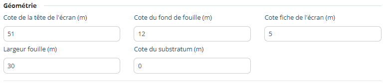
The geometry is defined based on the following data:
- Elevation of the top of the sheet pile (solely used for model visualization)
- Elevation of the excavation bottom
- Elevation of the sheet pile toe
- Width \(B_{max}\)
- Elevation of the substratum
Soil layers
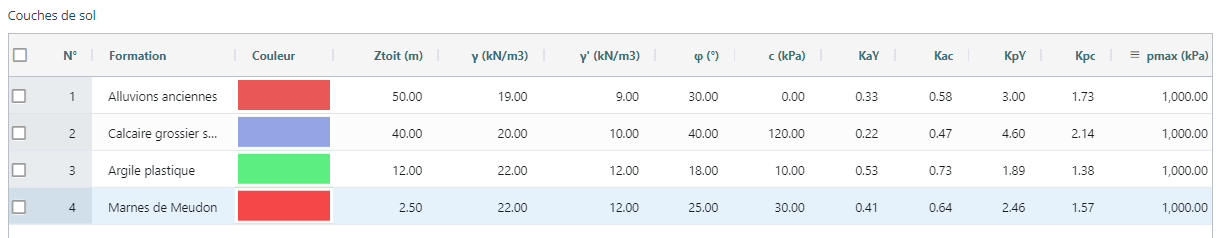
For each soil layer, it is necessary to define:
- \(Z_{top}\): elevation of the top of the layer
- \(\gamma\) (\(kN/m^3\)): total unit weight
- \(\gamma^{\prime}\) (\(kN/m^3\)): effective unit weight
- \(\varphi^{\prime}\) (°): effective friction angle
- \(K_{a\gamma}\): coefficient of horizontal active pressure
- \(K_{ac}\): coefficient of pressure applied to cohesion
- \(K_{p\gamma}\): coefficient of horizontal passive pressure
- \(K_{pc}\): coefficient of pressure applied to cohesion
- \(p_{max}\) (\(kPa\)): maximum pressure
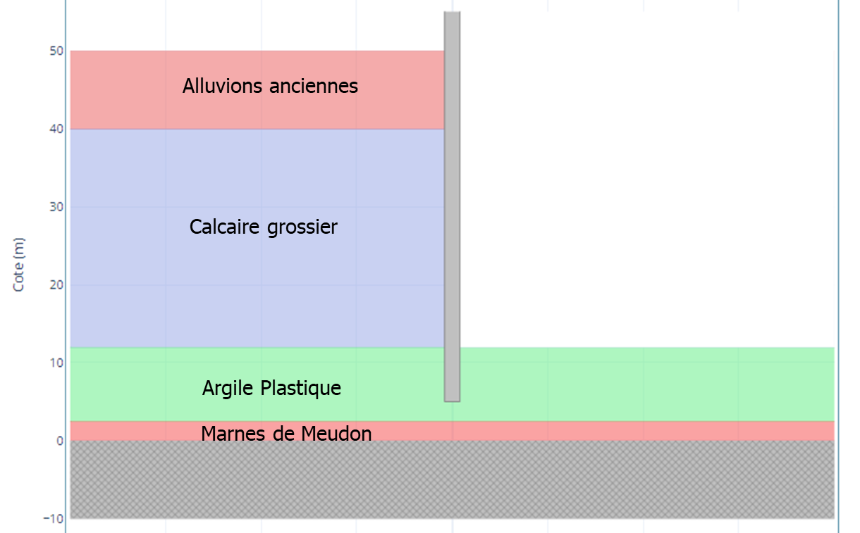
The geometric data is displayed in the model tab:
For your information
The calculation of the soil reaction under the foundation \(R(x)\) is performed with the cohesion, friction angle, and unit weight by volume of the layer directly beneath the toe of the sheet pile. In the example above, this corresponds to layer #3 of Plastic Clays. Any layer located below is not considered in the calculation (example of layer #4, Meudon Marl, here).
Calculation options

Equivalent volume weight of load-bearing soil
The equivalent weight by volume of the load-bearing soil \(\gamma^{*}\) is used to calculate the resistance \(R(x\)) and can be entered manually by the user.
For your information
By default ("Automatic" box checked), the equivalent weight by volume of the load-bearing soil γ* is taken to be equal to:
with :
-
\(x\) : the width of the examined mechanism
-
\(\Delta zw\) : depth of the water table relative to the elevation of the sheet pile
-
\(\gamma\) : wet density of the layer located directly under the toe of the sheet pile
-
\(\gamma^{\prime}\) : buoyant unit weight of the layer directly beneath the toe of the sheet pile
Note
The presence of the water table at an elevation \(z_w\) is automatically detected if a strictly positive hydrostatic pressure \(u\) is defined by the user at this elevation.
Thus, we have: \(\Delta z_w\) = Elevation of the screen sheet - \(z_w\).
Consideration of vertical shear
By default, the stabilizing forces associated with friction on the GL side or the excavation side are not taken into account in the calculation. The user can modify this option to take into account shear on the GL side only, or on both the GL and excavation side sides.
Calculation step
The default calculation step is 0.2 m and can be modified by the user.
Hydraulic Conditions and Overloads
Hydraulic Conditions
These tables allow defining the water table levels and possible gradients on the GL side (left of the screen) and on the bottom of the excavation (right of the screen).
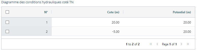
The parameters to be entered are :
- elevation (m): elevation \(z\) of the diagram point
- potential (m): potential \(h(z)\) to be taken into account for this point (the origin of the potentials is defined at coordinate \(z\) = 0 m).
The hydrostatic pressure \(u\) is calculated at each point: \(u(z) = (h(z) - z). \gamma_w\)
For your information
To define a water table, you need to provide at least two points corresponding to the top and base of the water table.
An hydrostatic water table is equivalent to a uniform potential (simply define two points with a potential \(h\) corresponding to the elevation \(z\) of the water table, as shown in the figure below):
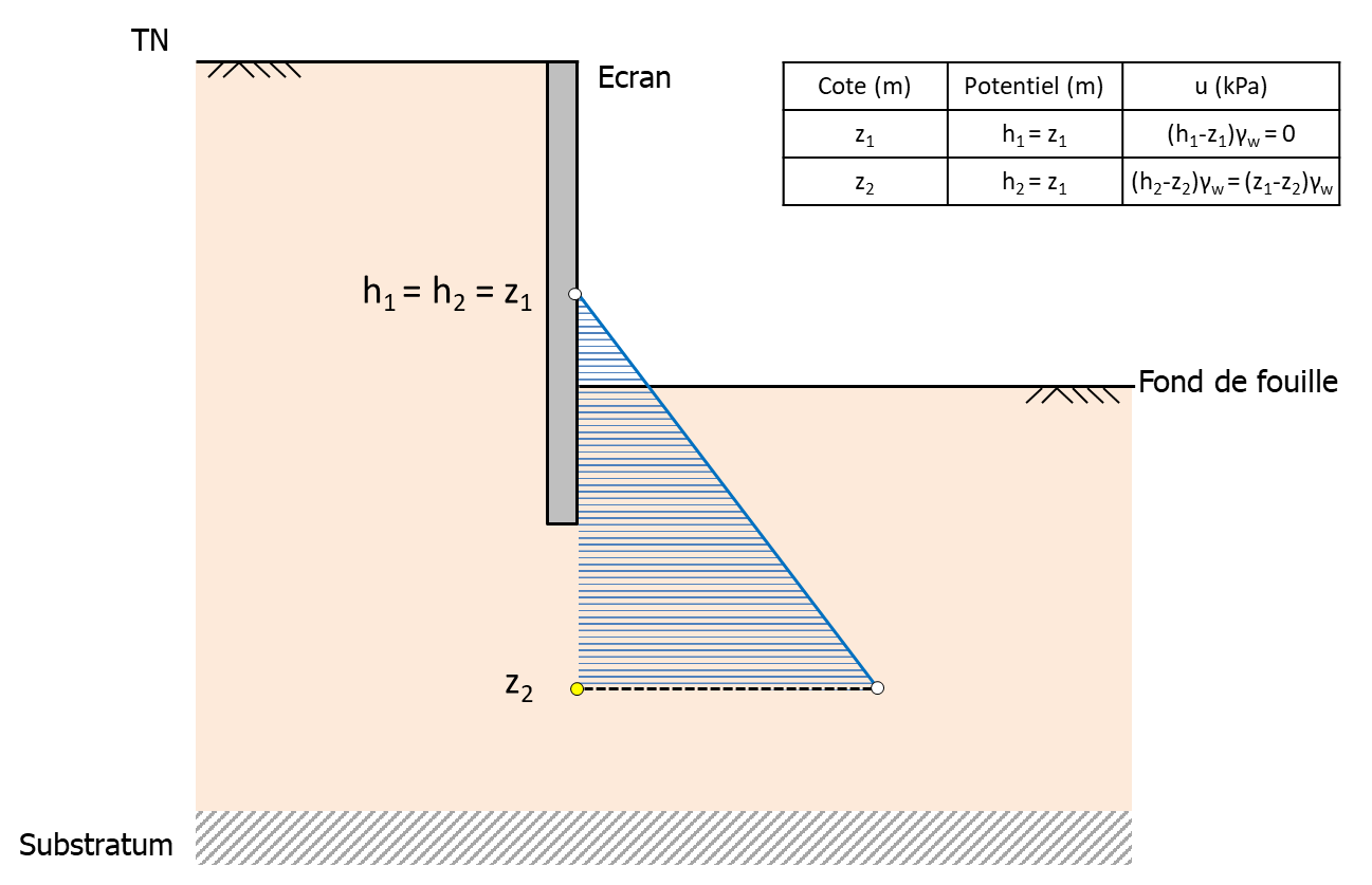
The presence of a gradient is equivalent to a variable potential \(h\). For this, you define a diagram (\(z_i\); \(h_i\)) with \(h_i\) varying with \(z_i\) as shown below:
For your information
In case of the absence of water, it is necessary to define a single point elevation/potential (for example, at the level of the substratum). In this case, the hydrostatic pressure is assumed to be zero at all elevations.
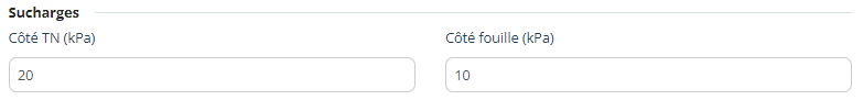
Loads
This section is used to define :
- The distributed load on the GL side (\(kPa\))
- The distributed load on the excavation side (\(kPa\))
Results
Main results
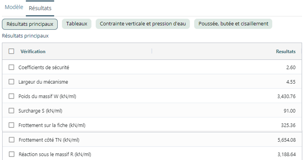
If the stabilizing forces related to vertical shear are taken into account in the "Calculation Options" section, the main results tab shows:
- \(F\) : the minimum safety factor
- \(x\) (\(m\)) : the width of the associated mechanism
- \(W\) (\(kN/ml\)) : destabilizing force due to the weight of the mass on the GL side
- \(S\) (\(kN/ml\)) : destabilizing force due to the surcharge on the GL side
- \(T_{sheet~pile}\) (\(kN/ml\)) : stabilizing force due to friction on the excavation side
- \(T_{GL}\) (\(kN/ml\)) : stabilizing force due to friction on the GL side
- \(R(x)\) (\(kN/ml\)) : reaction under the mass
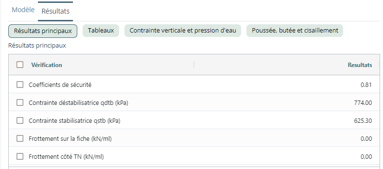
If the stabilizing forces related to vertical shear are ignored (default option), the width (\(x\)) of the mechanism does not play a role. The results tab then shows the safety coefficient :
where :
- \(q_{dtb}\) is the destabilizing stress such that:
- \(q_{stb}\) is the stabilising stress such that:
Tables
Tables tab presents:
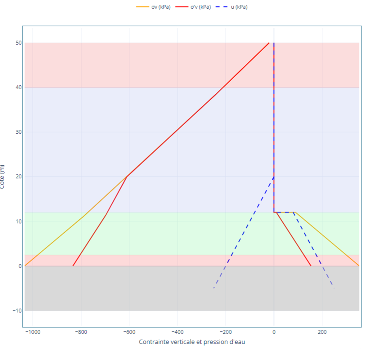
- \(σ_{v,F}\) (\(kPa\)): total vertical stress on the excavation side
- \(σ_{v,GL}\) (\(kPa\)): total vertical stress on the GL side
- \(σ^{\prime}_{v,F}\) (\(kPa\)): effective vertical stress on the excavation side
- \(σ^{\prime}_{v,GL}\) (\(kPa\)): effective vertical stress on the GL side
- \(u_F\) (\(kPa\)): water pressure on the excavation side
- \(u_{GL}\) (\(kPa\)): water pressure on the GL side
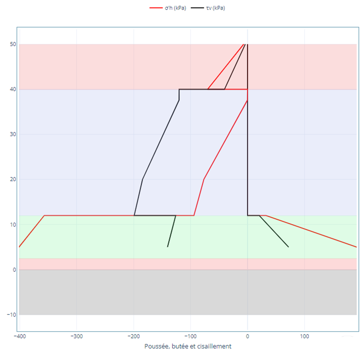
- \(\tau_F\) (\(kPa\)): shear stress on the excavation side
- \(\tau_{GL}\) (\(kPa\)): shear stress on the GL side

Graphics
The results are also presented in graphical format: